Identification of disease-associated cell states with MultiMIL

In this tutorial, we demonstrate how to train MultiMIL on the latent representation of an atlas. We will use the human lung cell atlas (HLCA) [SRSS+23], subset to healthy and idiopathic pulmonary fibrosis (IPF) samples.

We recommend the users always train MultiMIL on batch-corrected low-dimensional representations of the data.

The model will be trained in a binary classification setting, so we aim to predict healthy and IPF classes. We will obtain cell attention scores that are associated with the IPF samples and take a closer look at which cell states are most associated with the disease.

We also recommend the users to check out our sample-prediction pipeline, which includes MultiMIL and several other baselines, to assess whether the multiple-instance learning (MIL) approach is necessary for your use case or if pseudo-bulking or looking at cell type frequencies is sufficient to differentiate between classes.

import sys

# if branch is stable, will install via pypi, else will install from source
branch = "latest"
IN_COLAB = "google.colab" in sys.modules

if IN_COLAB and branch == "stable":
    !pip install multimil
elif IN_COLAB and branch != "stable":
    !pip install --quiet --upgrade jsonschema
    !pip install git+https://github.com/theislab/multimil

import multimil as mtm
import numpy as np
import scanpy as sc
import pandas as pd
import scvi
import warnings
from sklearn.model_selection import KFold

warnings.filterwarnings("ignore")

scvi.settings.seed = 0
print("Last run with scvi-tools version:", scvi.__version__)

Last run with scvi-tools version: 0.20.3

Data loading

We provide a subset of the HLCA containing healthy and idiopathic pulmonary fibrosis (IPF) samples. The data already contains the latent representations from the atlas.

data_path = "hlca_tutorial.h5ad"

try:
    adata = sc.read_h5ad(data_path)
except OSError:
    import gdown

    gdown.download("https://drive.google.com/uc?export=download&id=1wWGwbPeap-IqWNVlwVVUWVrUAMrf45ye")
    adata = sc.read_h5ad(data_path)

adata

AnnData object with n_obs × n_vars = 450214 × 30
    obs: "3'_or_5'", 'BMI', 'age_or_mean_of_age_range', 'age_range', 'anatomical_region_ccf_score', 'ancestry', 'assay', 'cause_of_death', 'cell_type', 'core_or_extension', 'dataset', 'development_stage', 'disease', 'donor_id', 'fresh_or_frozen', 'log10_total_counts', 'lung_condition', 'mixed_ancestry', 'sample', 'scanvi_label', 'sequencing_platform', 'sex', 'smoking_status', 'study', 'subject_type', 'suspension_type', 'tissue', 'tissue_coarse_unharmonized', 'tissue_detailed_unharmonized', 'tissue_dissociation_protocol', 'tissue_level_2', 'tissue_level_3', 'tissue_sampling_method', 'total_counts', 'ann_level_1_label_final', 'ann_level_2_label_final', 'ann_level_3_label_final', 'ann_level_4_label_final', 'ann_level_5_label_final'
    obsm: 'X_umap'

Data preparation

We will split the data into 3 cross-validation splits and check the prediction accuracy on the validation set to make sure that the model generalizes, which in turn means that the learned cell attention scores are also reflective of the disease.

Depending on how big your dataset is, i.e. how many samples there are, you might want to have 3 to 5 splits, but make sure that there is at least a few samples from each class in each of the validation splits so the prediction performance on the validation set can be assessed properly.

We will first walk through the steps required to train the model on one of the splits, and then we’ll repeat the steps for the other two splits before looking into detail at the cell attention scores.

sample_key = "sample"  # the smallest sample-level grouping variable, could be e.g. patient or sample (not batch)
disease_key = "disease"  # column containing disease labels, has to be the same value for all cells in a sample

We already subset the dataset to have a balanced number of samples in each of the classes. If your custom data has highly unbalanced class distribution, you might want to remove some of the less-represented classes or subset the classes with a lot of samples.

adata.obs[[sample_key, disease_key]].drop_duplicates().groupby(disease_key).size()

disease
normal                67
pulmonary fibrosis    67
dtype: int64

samples = np.array(adata.obs[sample_key].unique())
len(samples)

134

n_splits = 3
kf = KFold(n_splits=n_splits, shuffle=True, random_state=0)

for i, (train_index, val_index) in enumerate(kf.split(samples)):
    train_samples = samples[train_index]
    val_samples = samples[val_index]
    adata.obs.loc[adata.obs[sample_key].isin(train_samples), f"split{i}"] = "train"
    adata.obs.loc[adata.obs[sample_key].isin(val_samples), f"split{i}"] = "val"
    adata_train = adata[adata.obs[f"split{i}"] == "train"].copy()
    adata_val = adata[adata.obs[f"split{i}"] == "val"].copy()

    # check that all disease conditions in validation are present in training
    train_conditions = set(adata_train.obs[disease_key].unique())
    val_conditions = set(adata_val.obs[disease_key].cat.unique())
    assert val_conditions.issubset(train_conditions)

del adata_train, adata_val

query = adata[adata.obs["split1"] == "val"].copy()
ref = adata[adata.obs["split1"] == "train"].copy()

query.obs["ref"] = "query"
ref.obs["ref"] = "reference"

query

AnnData object with n_obs × n_vars = 161039 × 30
    obs: "3'_or_5'", 'BMI', 'age_or_mean_of_age_range', 'age_range', 'anatomical_region_ccf_score', 'ancestry', 'assay', 'cause_of_death', 'cell_type', 'core_or_extension', 'dataset', 'development_stage', 'disease', 'donor_id', 'fresh_or_frozen', 'log10_total_counts', 'lung_condition', 'mixed_ancestry', 'sample', 'scanvi_label', 'sequencing_platform', 'sex', 'smoking_status', 'study', 'subject_type', 'suspension_type', 'tissue', 'tissue_coarse_unharmonized', 'tissue_detailed_unharmonized', 'tissue_dissociation_protocol', 'tissue_level_2', 'tissue_level_3', 'tissue_sampling_method', 'total_counts', 'ann_level_1_label_final', 'ann_level_2_label_final', 'ann_level_3_label_final', 'ann_level_4_label_final', 'ann_level_5_label_final', 'split0', 'split1', 'split2', 'ref'
    obsm: 'X_umap'

Data setup

We need to specify which covariate will be our prediction covariate, so in this case it is disease that contains information whether each sample is a healthy or an IPF sample. The sample key is needed so the model knows which cells come from which sample.

The following step is compatible with the classification and ordinal regression setups, please refer to the regression tutorial.

classification_keys = [disease_key]
categorical_covariate_keys = classification_keys + [sample_key]

For the training to work properly, we need to sort the data by samples.

idx = ref.obs[sample_key].sort_values().index
ref = ref[idx].copy()

idx = query.obs[sample_key].sort_values().index
query = query[idx].copy()

mtm.model.MILClassifier.setup_anndata(
    ref,
    categorical_covariate_keys=categorical_covariate_keys,
)

Model setup and training

Next, we initialize the model. We need to specify the prediction covariate and the sample key. The prediction covariate and the sample key have to be registered covariates that we passed to setup_anndata() in the previous step. We set the coefficient for the classification loss here to 0.1. This parameter might require some fine-tuning depending on the dataset.

In case of an ordinal regression task, please specify ordinal_regression=classification_keys instead of classification=classification_keys.

mil = mtm.model.MILClassifier(
    ref,
    classification=classification_keys,
    sample_key=sample_key,
    class_loss_coef=0.1,
)

mil.train()

Epoch 51/200:  26%|██▌       | 51/200 [06:36<19:18,  7.78s/it, loss=2.98e-10, v_num=1]
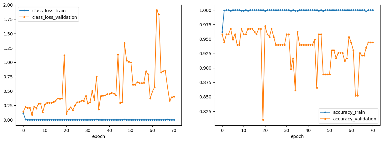
Monitored metric accuracy_validation did not improve in the last 50 records. Best score: 1.000. Signaling Trainer to stop.

mil.plot_losses()

Next, we obtain the learned attention scores; they are saved to .obs['cell_attn'] by default.

mil.get_model_output()
ref

AnnData object with n_obs × n_vars = 289175 × 30
    obs: "3'_or_5'", 'BMI', 'age_or_mean_of_age_range', 'age_range', 'anatomical_region_ccf_score', 'ancestry', 'assay', 'cause_of_death', 'cell_type', 'core_or_extension', 'dataset', 'development_stage', 'disease', 'donor_id', 'fresh_or_frozen', 'log10_total_counts', 'lung_condition', 'mixed_ancestry', 'sample', 'scanvi_label', 'sequencing_platform', 'sex', 'smoking_status', 'study', 'subject_type', 'suspension_type', 'tissue', 'tissue_coarse_unharmonized', 'tissue_detailed_unharmonized', 'tissue_dissociation_protocol', 'tissue_level_2', 'tissue_level_3', 'tissue_sampling_method', 'total_counts', 'ann_level_1_label_final', 'ann_level_2_label_final', 'ann_level_3_label_final', 'ann_level_4_label_final', 'ann_level_5_label_final', 'split0', 'split1', 'split2', 'ref', '_scvi_batch', 'cell_attn', 'bags', 'predicted_disease'
    uns: '_scvi_uuid', '_scvi_manager_uuid', 'bag_true_disease', 'bag_full_predictions_disease'
    obsm: 'X_umap', '_scvi_extra_categorical_covs', 'full_predictions_disease'

Predicting on the query samples

new_model = mtm.model.MILClassifier.load_query_data(query, mil)

new_model.get_model_output()
query

AnnData object with n_obs × n_vars = 161039 × 30
    obs: "3'_or_5'", 'BMI', 'age_or_mean_of_age_range', 'age_range', 'anatomical_region_ccf_score', 'ancestry', 'assay', 'cause_of_death', 'cell_type', 'core_or_extension', 'dataset', 'development_stage', 'disease', 'donor_id', 'fresh_or_frozen', 'log10_total_counts', 'lung_condition', 'mixed_ancestry', 'sample', 'scanvi_label', 'sequencing_platform', 'sex', 'smoking_status', 'study', 'subject_type', 'suspension_type', 'tissue', 'tissue_coarse_unharmonized', 'tissue_detailed_unharmonized', 'tissue_dissociation_protocol', 'tissue_level_2', 'tissue_level_3', 'tissue_sampling_method', 'total_counts', 'ann_level_1_label_final', 'ann_level_2_label_final', 'ann_level_3_label_final', 'ann_level_4_label_final', 'ann_level_5_label_final', 'split0', 'split1', 'split2', 'ref', '_scvi_batch', 'cell_attn', 'bags', 'predicted_disease'
    uns: '_scvi_uuid', '_scvi_manager_uuid', 'bag_true_disease', 'bag_full_predictions_disease'
    obsm: 'X_umap', '_scvi_extra_categorical_covs', 'full_predictions_disease'

To be able to access the cell attention scores after the training for the other two splits, we also save them in .obs['cell_attn_0'] in the original adata object.

cell_attn_0 = pd.concat([ref.obs["cell_attn"], query.obs["cell_attn"]])
cell_attn_0.name = "cell_attn_0"

adata.obs = adata.obs.join(cell_attn_0)

We can also calculate the prediction accuracy for the query samples. Here, we calculate it on the cell level, where the prediction for each cell was copied over from the sample prediction. It’s only possible to calculate the prediction on the bag level by accessing the bag prediction stored in query.uns['bag_full_predictions_disease']. In our experience, the cell-level prediction accuracy differs very little from the bag-level prediction accuracy.

from sklearn.metrics import classification_report

print(classification_report(query.obs[disease_key], query.obs[f"predicted_{disease_key}"]))

                    precision    recall  f1-score   support

            normal       0.99      0.91      0.95     59029
pulmonary fibrosis       0.95      1.00      0.97    102010

          accuracy                           0.96    161039
         macro avg       0.97      0.95      0.96    161039
      weighted avg       0.97      0.96      0.96    161039

Putting all together for the rest of the splits

Next, we perform the training for the other two splits. We recommend the users to use the code snippet from the following cell and run it for all the splits in their analysis.

for i in range(1, n_splits):  # change to range(n_splits) to run all splits
    print(f"Processing split {i}...")
    query = adata[adata.obs[f"split{i}"] == "val"].copy()
    ref = adata[adata.obs[f"split{i}"] == "train"].copy()

    query.obs["ref"] = "query"
    ref.obs["ref"] = "reference"

    idx = ref.obs[sample_key].sort_values().index
    ref = ref[idx].copy()

    idx = query.obs[sample_key].sort_values().index
    query = query[idx].copy()

    mtm.model.MILClassifier.setup_anndata(
        ref,
        categorical_covariate_keys=categorical_covariate_keys,
    )

    mil = mtm.model.MILClassifier(
        ref,
        classification=classification_keys,
        sample_key=sample_key,
        class_loss_coef=0.1,
    )

    mil.train()

    mil.get_model_output()

    new_model = mtm.model.MILClassifier.load_query_data(query, mil)

    new_model.get_model_output()

    cell_attn_i = pd.concat([ref.obs["cell_attn"], query.obs["cell_attn"]])
    cell_attn_i.name = f"cell_attn_{i}"

    adata.obs = adata.obs.join(cell_attn_i)

    print(classification_report(query.obs[disease_key], query.obs[f"predicted_{disease_key}"]))

Processing split 1...
Epoch 51/200:  26%|██▌       | 51/200 [05:32<16:11,  6.52s/it, loss=2.09e-09, v_num=1]
Monitored metric accuracy_validation did not improve in the last 50 records. Best score: 1.000. Signaling Trainer to stop.
                    precision    recall  f1-score   support

            normal       0.78      0.89      0.83     59029
pulmonary fibrosis       0.93      0.86      0.89    102010

          accuracy                           0.87    161039
         macro avg       0.86      0.87      0.86    161039
      weighted avg       0.88      0.87      0.87    161039

Processing split 2...
Epoch 51/200:  26%|██▌       | 51/200 [06:02<17:38,  7.11s/it, loss=3.28e-09, v_num=1]
Monitored metric accuracy_validation did not improve in the last 50 records. Best score: 1.000. Signaling Trainer to stop.
                    precision    recall  f1-score   support

            normal       1.00      0.96      0.98     77812
pulmonary fibrosis       0.95      1.00      0.97     63059

          accuracy                           0.97    140871
         macro avg       0.97      0.98      0.97    140871
      weighted avg       0.97      0.97      0.97    140871

Cell attention scores and sample representations

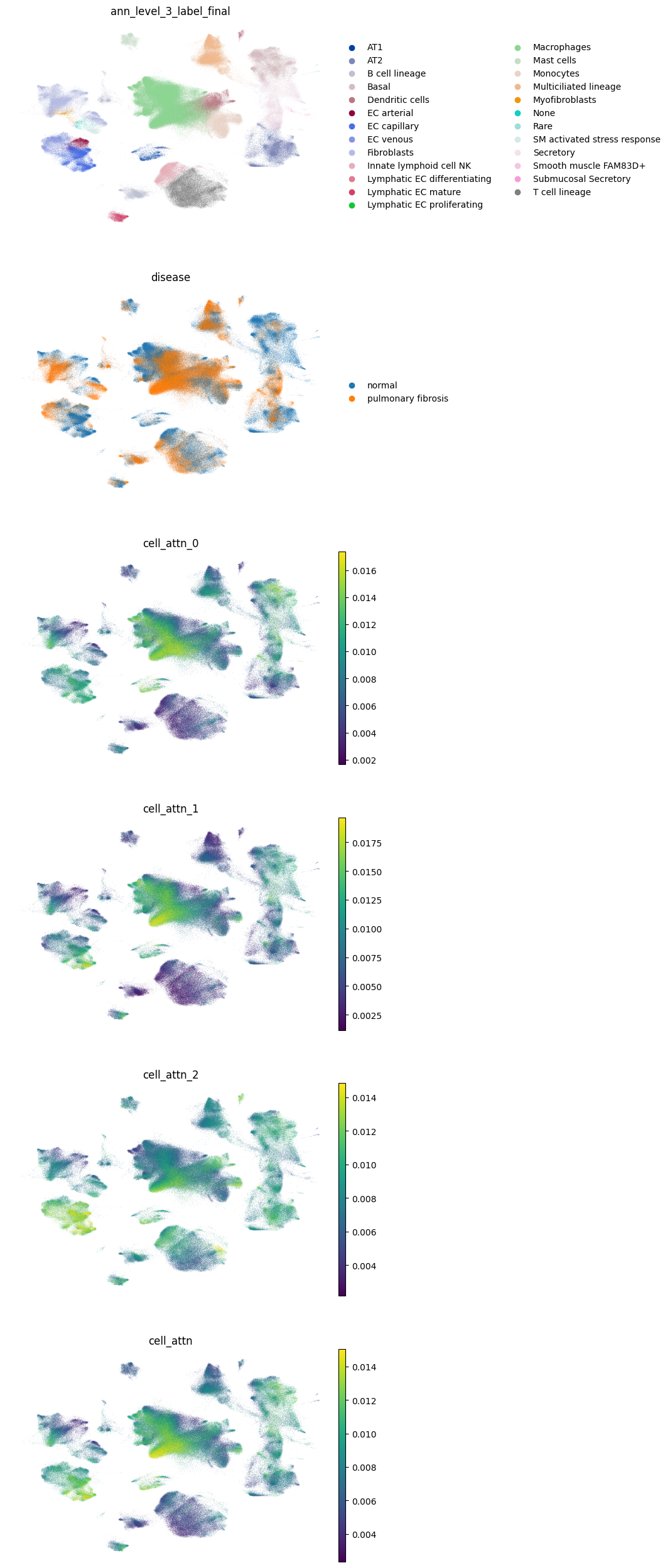
We check the consistency of the attention scores per split and use the averaged scores for downstream analysis and sample representation calculation.

adata.obs["cell_attn"] = np.mean(adata.obs[["cell_attn_0", "cell_attn_1", "cell_attn_2"]].values, axis=1)

sc.pl.umap(
    adata,
    color=["ann_level_3_label_final", "disease", "cell_attn_0", "cell_attn_1", "cell_attn_2", "cell_attn"],
    ncols=1,
    frameon=False,
    vmax="p99",
)

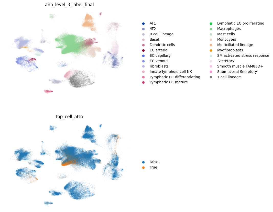
Next, we identify cells with high attention scores (top 10%) and save this information into a new column to .obs. We recommend using the cells with high attention per disease class for downstream analyses, such as differential expression testing, e.g. between high-attention disease cells vs healthy or high-attention disease cells vs all disease cells.

mtm.utils.score_top_cells(adata)  # uses .obs['cell_attn'] by default

sc.pl.umap(
    adata[adata.obs[disease_key] == "pulmonary fibrosis"],
    color=["ann_level_3_label_final", "top_cell_attn"],
    ncols=1,
    frameon=False,
)

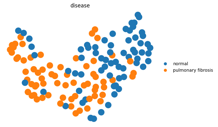
Finally, we use the cell attention scores to calculate the sample representations as a weighted sum of cell representations for each sample.

sample_reps = mtm.utils.get_sample_representations(adata, sample_key=sample_key, covs_to_keep=[disease_key])
sample_reps

AnnData object with n_obs × n_vars = 134 × 30
    obs: 'disease'

sc.pp.neighbors(sample_reps, n_neighbors=10)
sc.tl.umap(sample_reps)

sc.pl.umap(
    sample_reps,
    color=[disease_key],
    ncols=1,
    frameon=False,
)